Designing an Audio Anomaly Detector Using the Neyman-Pearson Lemma
Suppose you are an engineer who was asked to detect intruders on your granny’s farm. Being the resourceful engineer, you decide to bury a cheap USB microphone in a junction box by the only entrance of the farm. The plan is simple: if someone walks or drives in during the night, the cops will be automatically alerted. Our primary goal is, therefore, to design a detection algorithm that maximizes the odds of detecting intruders. Since we obviously don’t want to inconvenience the cops, our secondary goal is to minimize the number of false alarms.
Fortunately, half of this is a solved problem. In this article, we will be walking through the entire thought process, arming ourselves with the fields of Statistics, Data Science, and Detection Theory.
Initial Exploratory Analysis
Not only are you an engineer, you also double as a data scientist! Because of these skills you know that one of the most important steps in solving any data science problem is to visualize and understand the data as much as you can. So, you take your cheap microphone, plug it into your cheap computer, and, after a quick scripting session, you get the following plot:
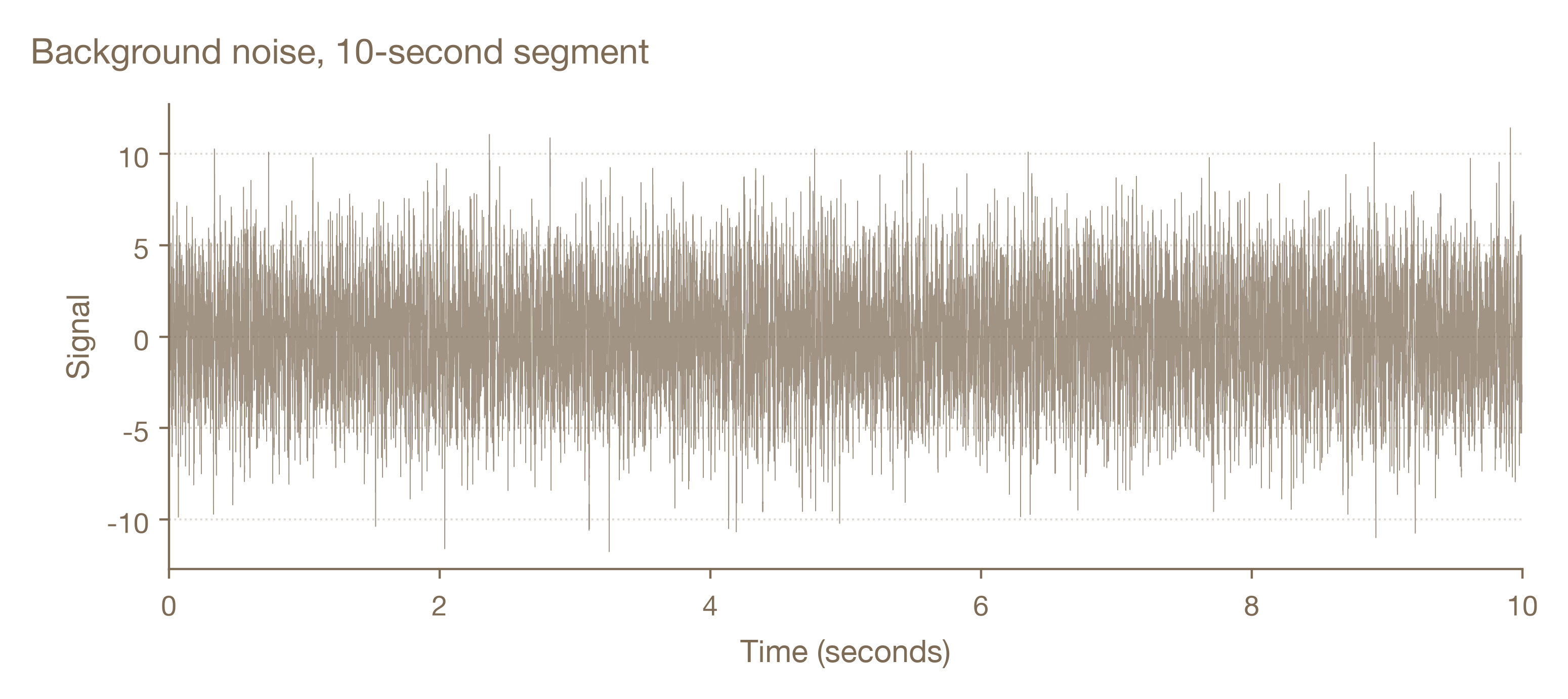
This is the plot you get when you captured absolute silence. It is not a constant 0 because it likely includes electronic noise and unnoticeable sounds. Within 10 seconds, your cheap microphone produced 80k samples, which means its sampling frequency is \(f_s = 8\,\text{kHz}\), a typical value for a voice-grade mic. Looking at the plot, the engineer in you is screaming “This is White Gaussian Noise!” (WGN), while the data scientist in you is yelling back “Let’s see what the distribution looks like before jumping to conclusions!”. Fortunately, you listened to the data scientist, and, after some more intense scripting, you come up with the plots below:
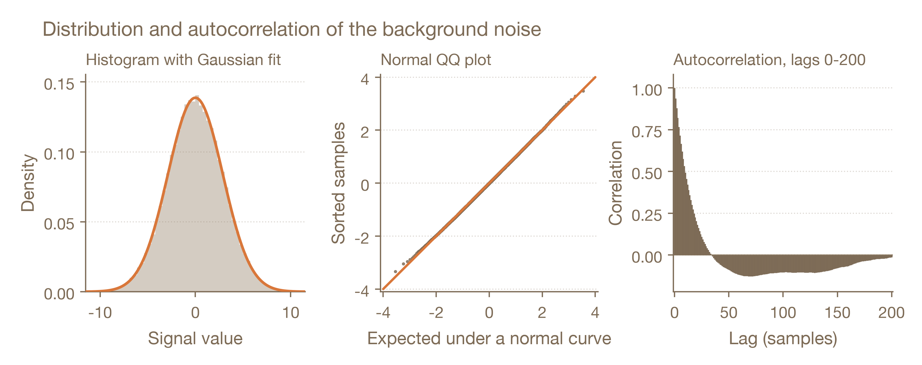
Very interesting! Not only does your PDF (Probability Density Function) look like a Gaussian curve, the QQ plot confirms that we’re working with a Gaussian. However, interestingly enough, the autocorrelation function (ACF) plot indicates that our signal’s samples are not independent of each other — that is, the signal’s next value depends on its previous values. This is an interesting behavior, likely caused by some filtering mechanism in the microphone.
Alright! With noise data profiled, it’s time to understand what happens to the microphone signal when intruders try to break into the farm. Putting on the scientist hat, you design a data collection experiment that tests 3 distinct situations near the microphone: (i) a pickup truck driving by, (ii) a person walking near it, and (iii) a cat sneaking around. You manage to organize the whole ordeal, recording 1 minute of data where the 3 events happen:
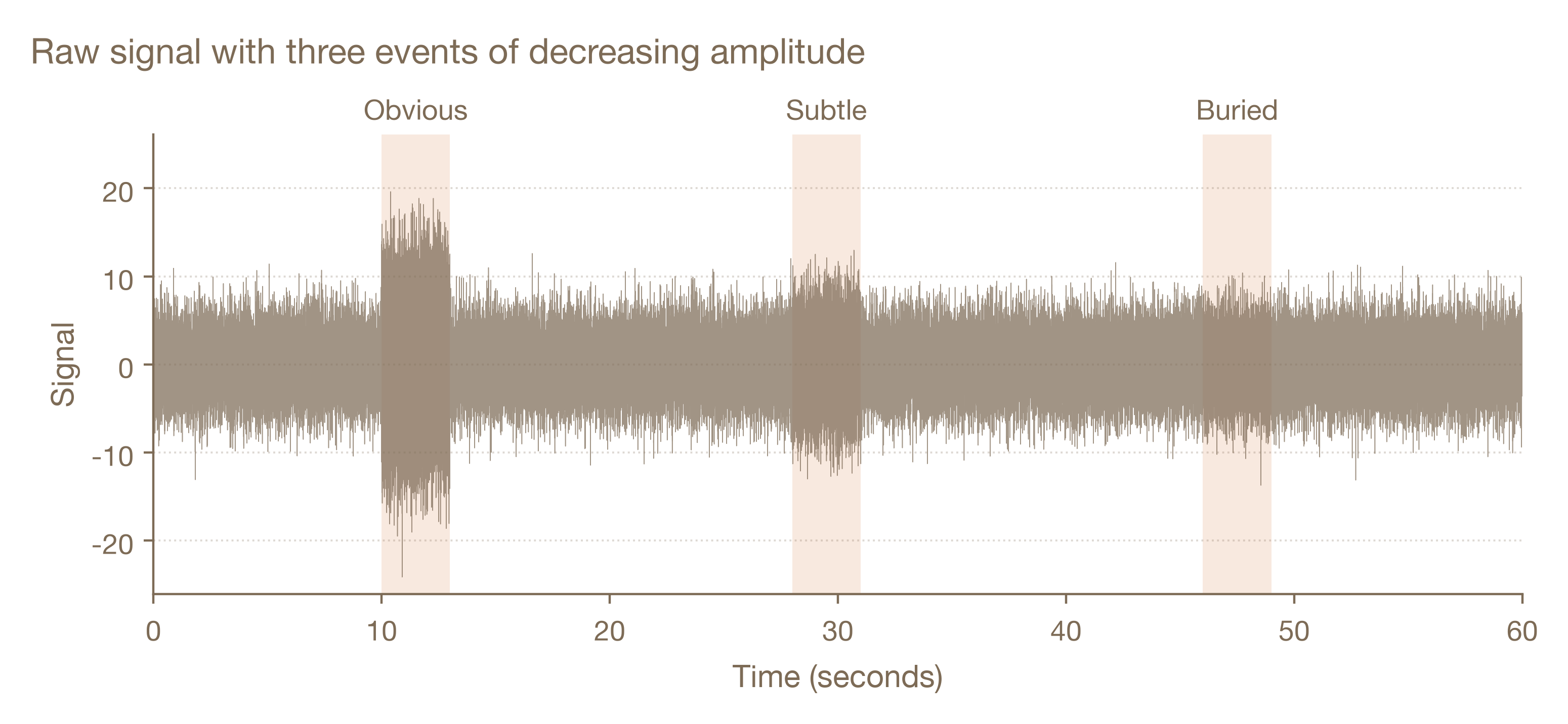
As it turns out, we can clearly identify the truck in the signal, while the person signal is barely noticeable — and the sneaky cat will still be able to invade granny’s farm. That’s ok, we don’t mind small visitors, and the cat is probably keeping some pests away. Unfortunately for you, the signal of a person walking by the microphone is very weak relative to the baseline noise. If we want to design a good detection algorithm, we are in for a challenge.
Among other things, you are also a humble engineer. You understand that people smarter than you have probably solved similar problems already, so you decide to turn your attention to the literature. After nagging the local librarian a bit, you discover the field of Detection Theory and decide to read the book Fundamentals of Statistical Signal Processing, Volume II: Detection Theory, by Steven M. Kay. This is a great find, because, apparently, your problem is a classic textbook problem.
When thinking about designing a detector, you initially think of simple threshold methods. For example: if the signal crosses \(+T\) or \(-T\), trigger a detection. You immediately discard this idea, because an intruder doesn’t produce one big sample; it produces thousands of slightly bigger ones. Then, you think of different ways to measure signal variability: amplitude, standard deviation, zero-crossing rate, even spectral energy. What if, instead, there were a mathematically proven method to solve this problem?
You stumble across the Neyman-Pearson lemma and how it can be used to derive what is called the Uniformly Most Powerful (UMP) hypothesis test. You immediately use it for our problem: assuming that both noise and signal data are normally distributed with 0 mean (\(\mathcal {N}(0 ,\sigma ^{2})\)), we test for \({H_{0}:\sigma ^{2}=\sigma _{\text{noise}}^{2}}\) against \({H_{1}:\sigma ^{2}=\sigma _{\text{intruder}}^{2}}\). This derivation, however, assumes the samples are independent, while the ACF plot says they aren’t. You ignore this small detail, but it will bite you later.
By the Neyman-Pearson lemma, the UMP test for this case depends only on \({\hat{s}^{2} = \sum _{i=1}^{n}x_{i}^{2}}\), which is essentially the signal energy/variance! A clear, interpretable result. You decide to call the statistic \(\hat{s}\) the signal’s loudness. Now all you have to do is set a window size \(n\) and a threshold \(T\) that, when crossed by \(\hat{s}\), triggers the detector.
You quickly run back home, select \(n=8000\) samples (corresponding to a single second), normalize \(\hat{s}\) so a usual quiet second reads \(1.0\), eyeball an arbitrary threshold \(T = 1.07\), and test it against your data. You generate the figure below:
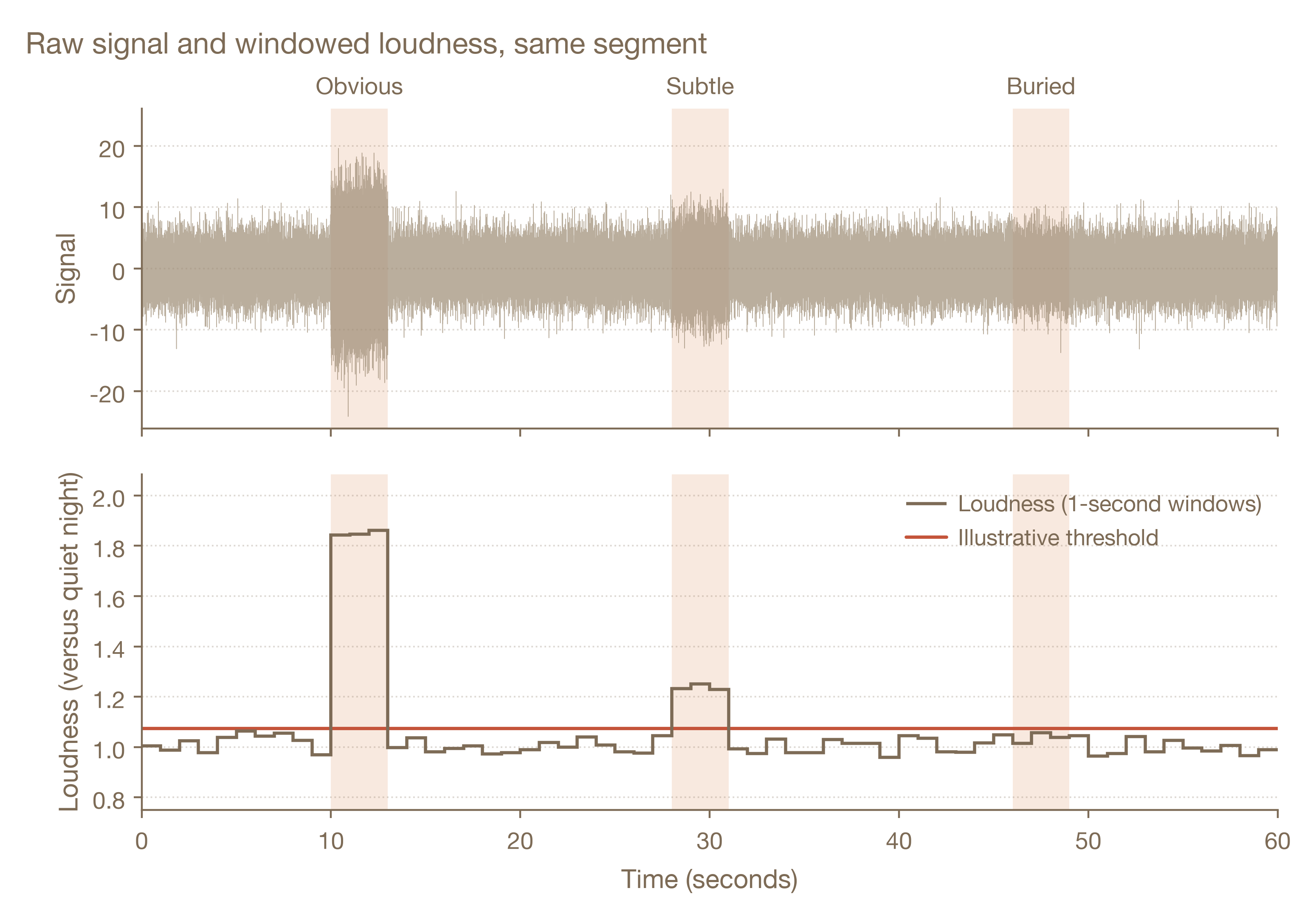
Look at that! The truck towers over the threshold, as expected, but the person, nearly invisible in the raw signal, shows cleanly above the line too. The statistic caught an intruder our eye couldn’t. Only the cat stays hidden, and there is nothing to do about that (unless you buy an expensive microphone, but granny won’t like that idea). It seems like our primary objective has been met.